S-distortion Correction and Wavelength Calibration (Step=5)
Relevant code
XDpiped.csh SdistorAndWLcalibXD.py
Relevant options
1nssdist_inter: yes/no (no) [run nssdist interactively?]
2nswav_inter:   yes/no (no) [run nswavelength interactively?]
3nsfit_inter:   yes/no (no) [run nsfitcoords interactively?]
What it does
XDpiped.csh now calls the SdistorAndWLcalibXD.py module, which uses the
nssdist, nswavelength, nsfitcoords and nstransform tasks to
rectify and wavelength-calibrate the data. This is what happens:
nssdist is used to find and trace the pinholes in the daytime pinhole flat.
nsfitcoords is run, using the results from nssdist, to provide the information that nstransform needs to straighten the spectral orders.
nstransform is run on the combined arc spectra. After this step the spectral orders are vertical, but the slight tilt of the detector means that the spatial direction is still not exactly parallel to the detector rows.
nswavelength is run on the straightened arc to obtain the pixel-wavelength relation. nswavelength is called with
fl_median-, which causes it to call nsfitcoords and nstransform, and (temporarily) produce an arc with horizontal arc lines.nsfitcoords and nstransform are run on the straightened arc.
This series of events provides the information necessary to rectify the
orders in the science target and standard star data, and then de-tilt
the data so that the spatial direction is along the detector rows.
Usually, nsfitcoords would be run on each file to provide
the information necessary for nstransform to rectify the data. However,
the output from nsfitcoords is based on only the arc and pinhole data,
which are the same for every on-sky data file. XDGNIRS therefore
contains a hack to edit the headers to link the data to the
nsfitcoords solution from steps 2 and 5 in the database files,
eliminating the need to run the task multiple times. However, Nstransform is
still run twice on each file, first to straighten the orders and then to
perform the slight de-tilting. This is a fairly complex process, and the
curious user can inspect the tf\* and ttf\* files to see how the data
change at each step.
What to look for
Check that the final, combined files (e.g., standard_comb.fits) look
reasonable. It is usually quite obvious when things have gone wrong, but
sometimes more subtle problems are present, such as the slit appearing
to change in length by a few pixels along the order. A 1D,
wavelength-calibrated arc spectrum is also generated at this stage
(calibrated_arc.fits), and can serve as a useful sanity check of the
wavelength calibration. In addition, the code compares the actual
wavelength coverage with the expected coverage and writes the results
into the Checks_and_Warnings.txt file. The calculation is specifically
for \(\lambda_{cen}\)=1.65 \(\mu\)m, and should be ignored
for other central wavelengths.
Things to most likely go wrong
Sometimes a wavelength solution is not found, (hopefully) causing the code to
exit with an error. This often means that one or more orders have not been
appropriately transformed. If that is the case, that order in the transformed
files (ttf*fits) or final, combined files – target_comb.fits,
standard_comb.fits; see Combining the Files (Step=6), will look odd (perhaps exhibiting
what we call the “snake effect,” which is probably self-explanatory). This can
usually be fixed by restarting from this step with nssdist_inter=yes or
nsfit_inter=yes, and deleting deviant points in nsfitcoords (as described
on the GNIRS XD web page).
If the transformed data look good, it may be that nswavelength cannot
automatically find a wavelength solution. Use nswav_inter=yes to see if there
is an obvious problem, or inspect the reduced arc files. Offsets between
quadrants in the arcs can upset nswavelength, as can arcs with no lines
(because of a problem with the arc lamp or other mechanism (an uncommon
occurrence). Occasionally, it is necessary to manually identify some lines for
no apparent reason.
Example: NGC 3031
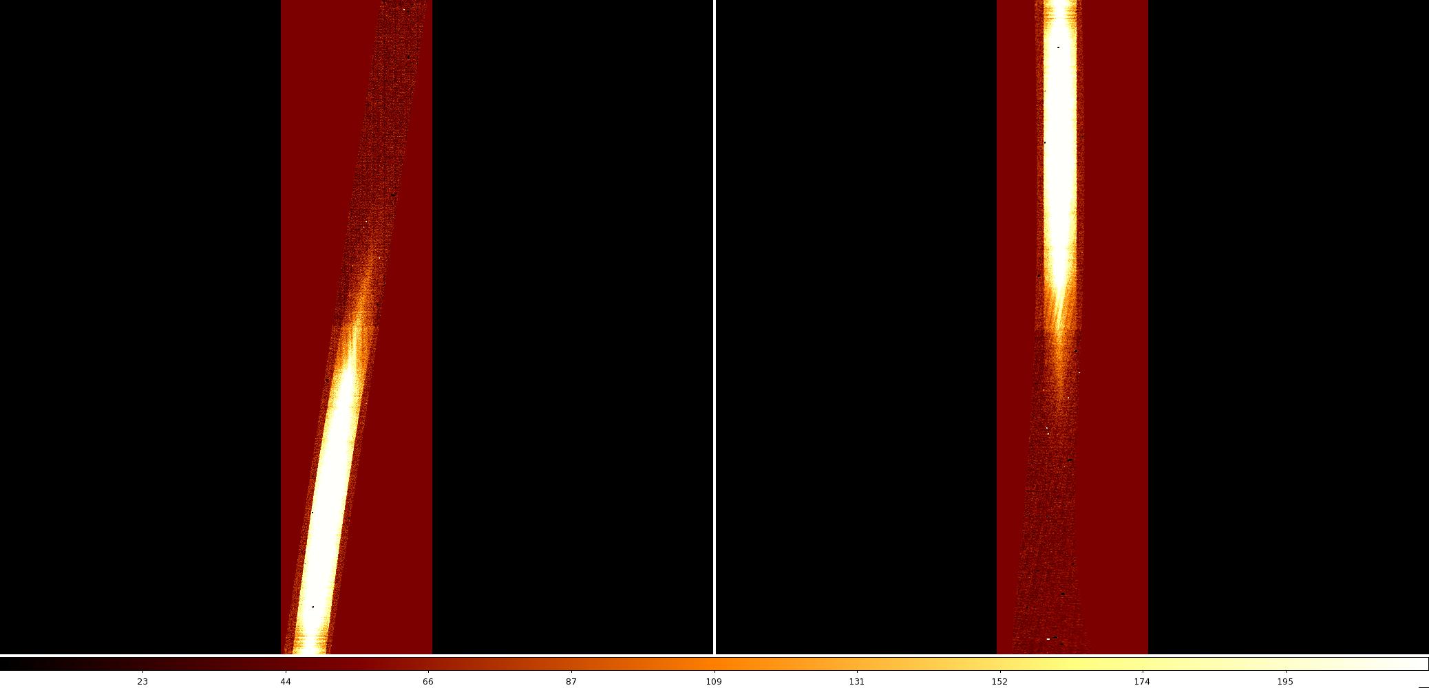
Two orders of the NGC 3031 spectra are shown in Fig. 7 and Fig. 8, before and after running nstransform on the science data. The wavelength initially increases from top to bottom, the orders are tilted, and the sky lines are not exactly parallel to the detector rows. In the transformed data set, the wavelength scale is flipped, the orders are vertical, and the sky lines are horizontal to within 0.2 pixels. The short-wavelength end of order eight has not been well rectified, but this is because the throughput in that region is low enough that even the pinhole flats have little signal. There are no useful science data in that region, so the odd shape is not a problem. The same is true for smaller portions of orders 6 and 7.
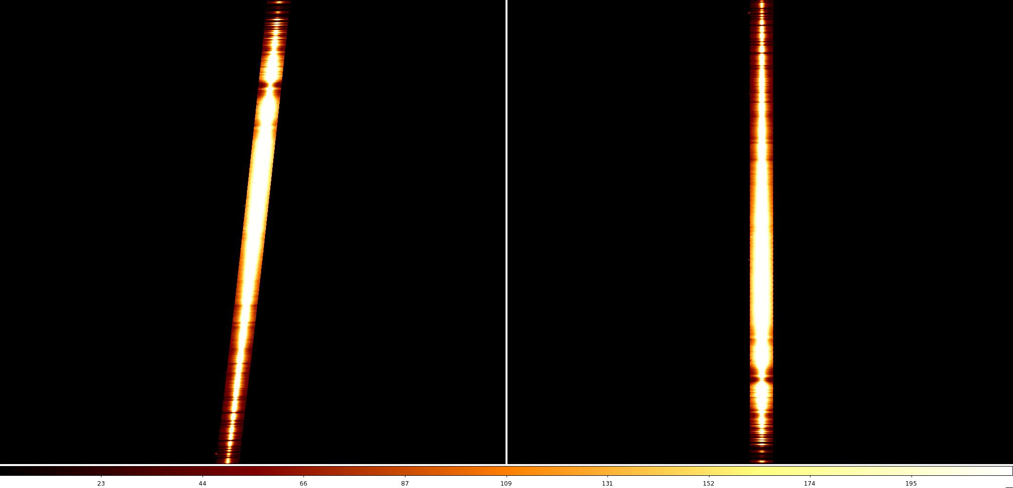
Fig. 7 Extension1/order3 before and after transforming (files rlncN20120305S0067, ttfrlncN20120305S0067; z1=0, z2=200).